Word Embedding

Think about language input, e.g. a movie review about Interstellar.

The text first should be converted into numeric vectors.

Or image inputs, e.g. handwritten images of numbers.

The classification may be about whether the data sample is positve/negative or, out of 0-10, which number the image is reprensenting.

The text may be more challenging, as they have these so-called word dependencies between words. The longer the text, the more complicated the dependencies within them get.

So, we need a good conversion from text to vectors, and build a good neural networks (the mapping into the given classification layer).

One-hot Vector/Encoding

Given a corpus of text, we can get the vocabulary from it (consisting of unique terms), then we set the target vector dimenstion to represnet them. If you use the one-hot encoding, the dimension is equal to the size of the vocabulary. So if your vocab are 10, then the dimension is 10. e.g. “apple” becomes 0000000001 and “banana” becomes 0000000010. Only one index is assigned with value “one”, so one-hot!

Drawbacks of One-hot Representation

Curse of Dimenstionality

Many ML problems become exceedingly difficult when the number of dimensions in the data is high.

Each data sample is sparsely represented.

Information quality gets worse, memory use gets bigger, and computation time gets higher as your dimension gets bigger.

* usually 300 is popular dimension, e.g. Word2Vec.

Orthogonality

If you multiply two one-hot embeddings, you get always get zero. That may means all the two words is euqlly distances in terms of their similarity. e.g. the distance between “dog” and “puppy” is the same as “dog” and “computer”.

This can be called that all word embeddings are orthogonal to each other. We don’t want this for the downstream NLP tasks. We want numeric operations over them, assuming they are embedded in a semantically meaningful way.

Dimensionality Reduction

Due to the curse of dimension, we need to reduce the dimension.

The process of converting a set of high dimenstional data into a lower dimenstional representation that conves similar information.

E.g. Pricipal Component Analysis (PCA), Linear Discrimina Analysis (LDA)

PCA finds a linear subspace that maximized the variance of the data once it is projected into a lower-dimensitonal space. It also minimizes the distance off the projection in a least-squares sense.

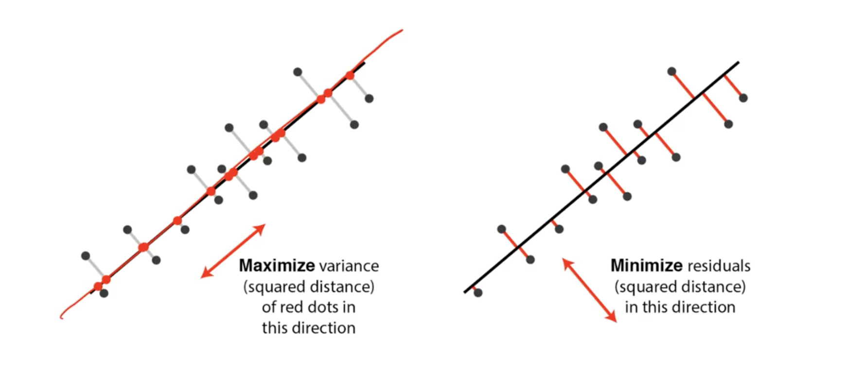
It means that while the data points gets maixmal variance (so that they are well distinguished from each other), we want to keep the pattern intact (the line in the right image well represent the dots!). SO we use the line (or a hyperplane) to replace the dots, reducing a dimension.

Manifold Hypothesis

PCA may be good. But problems get harder and harder as data forms non-linear patterns.

Manifolds hypothesis assumes that natural data often form the non-linear patterns.

Natural data in high dimensional spaces concentrates close to lower dimensional manifolds. Moving away from the supporting manifold (reducing dimension), probability density decreases (model becomes incorrect).

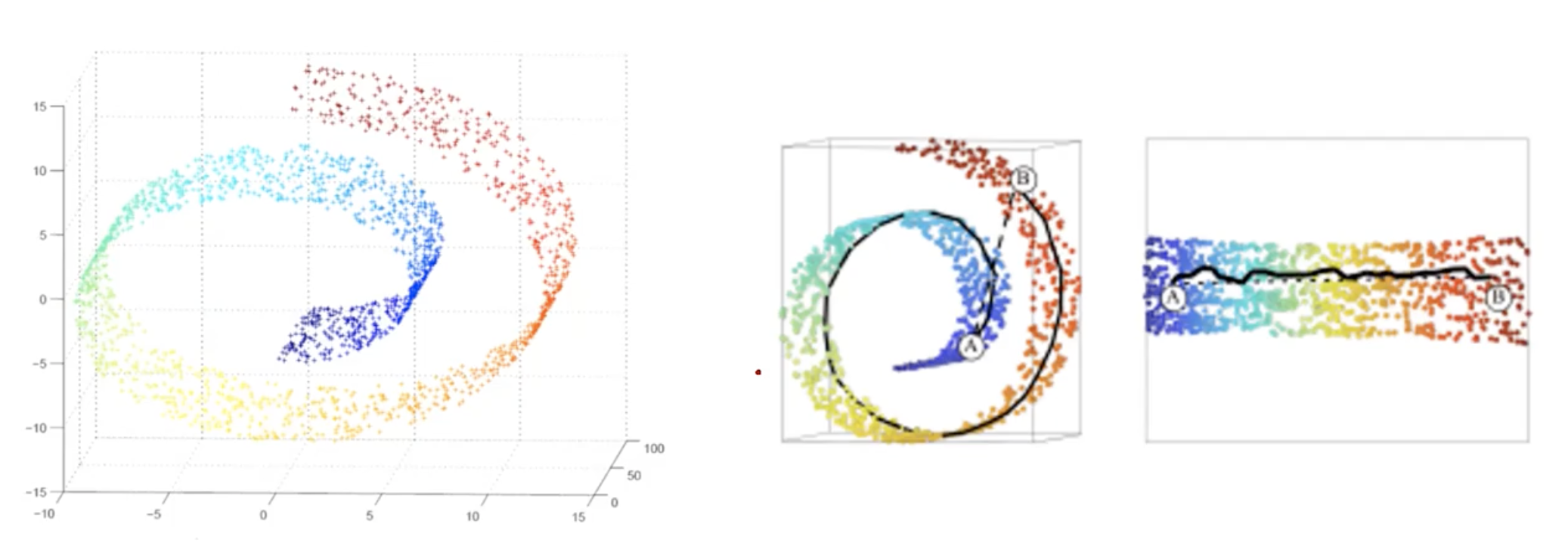
Reducing dimension in the middle image, the distance between two points A and B, gets very bigger. This may cause problems.

So dont’ just linearize the pattern in manifold patterns (instead of uniform patterns, or etc).

Regarding the words, are they form the manifold pattern? or maybe uniform patterns?

Autoencoder

Autoencoder is a neural network designe to learn an identity function in an unsupervised way to reconstruct the original input while compressing the data in the process so as to discover a more efficient and compressed representation.

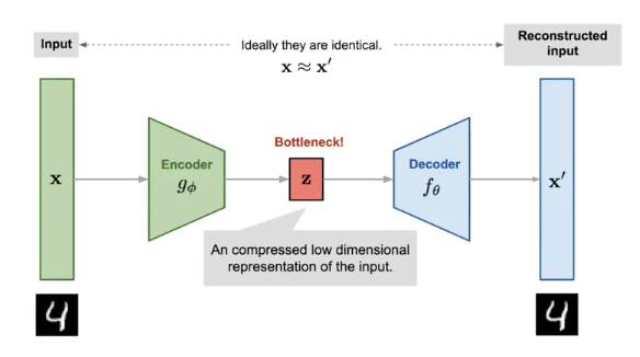
The autoencoder was proposed by Geoffrey Hinton, that aims to learn a very good representation in a unsupervised way - it compress the data into lower dimension (in to the bottleneck!) that can be reconstructed into the original data.

This arichtecture design use the bottleneck-based encoder & decoder two networks that accurately reconstruct the data but also reduce the size of dimension!

As the variants of this vanilla autoencoder was proposed, of course, e.g. auto-encoder into bigger dimension, note that this reconstructable & compressed chracteristic of autoencoder is not concrete.

It uses mean square error as its loss function usually, as they are regarded as ‘reconstruction error’.

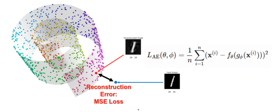
The intuition behind this function is how original data x is different of the x that is encoded and decoded to be reconstructed.

The bottlenec dimension may be, for example, 3 dimensional space. That is, any high-dimensional manifold can be represented into a lower dimension manifold.

When you’re finished the auto-encoding phase, you take the bottleneck represenatation as the input feature to the downstream task, which sounds reasonable, as they are reduced and reconstructable. Conventionally, autoencoder use small number of layers, such as 2: one for encoder and the other for decoder.

However, the advances in supervised deep learning (e.g. deeper layers, residual connections, ..), autoencoder is now that popularly used. Just use better model architecture that auto-encode (efficeint data codings) and solve the task.

Back to Drawbacks of One-hot Representation

1. Curse of dimensionality
2. Orthogonality

But let’s think if the autoencoder can succefully address these two problems, when used on one-hot encoded data.

For the former issue, yes, it may reduce the dimension. But for the latter issue, the orthogonality issue, whether the data is encoded in a way that the semantic dependence between words (one-hot) are encoded, not just word-independent embedding, is unlikely be solved via the autoencoder. There are no design to tackle this inter-word dependent relationsip!

Word2Vec

We move on to the main part of word embedding!

Another hypothesis over manifold hypothesis used for Autoencoder: Distributional Hypothesis.

“Tell me who your friedns are, and I will tell you who you are.”

Let’s say we want to encode a word “Trump”

The surroundings terms that is frequently used with “Trump” would be like “President”. That is the surroundings of word defines the meaning of words. It aims to encode the words by its frequency (statistical distribution) of the cooccurence in sentences, not by some fancy dimensionality analysis.

Continuous Bag of Words (CBOW)

Given a set of neighobring words (contexts), predict single words that potentially occur along with the contexts.

For example of our Trump, let’s say we see a sentence below,

“… and military officials, President Trump said yesterday, The United States is ready … “

Then the CBOW aims to predict which word is most likely to be occur between “President” and “said”

As we observed the sentence, “Trump” would be appropriate.

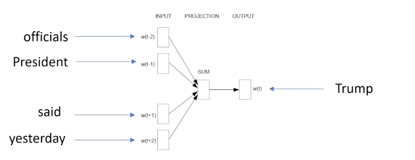
Here, as the candidate vocaluralies are enormously huge, we regard that there are a hypotheical finite set of words to consider the potential max pool of words. As, the ground truth label in CBOW is usually one-hot, the output of network will the dimension, same with the size of the vocabularies.

What’s the difference to autoencoder?

(The size of vocabulary) Although the both use is one-hot labelling, the prediction representations in CBOW are embedded in a contextual way. (there may be a reduced output representation which we’ll soon cover, but hypothesis behind this CBOW is considering all words as one-hot representation.)

What’s another issue?

(The size of window) How wide the context should be, when we are trying to teach the most likely word in between?

Word2Vec: CBOW

Formally these two concerns hyperparameterized the shape of learnable matrix W: NxV

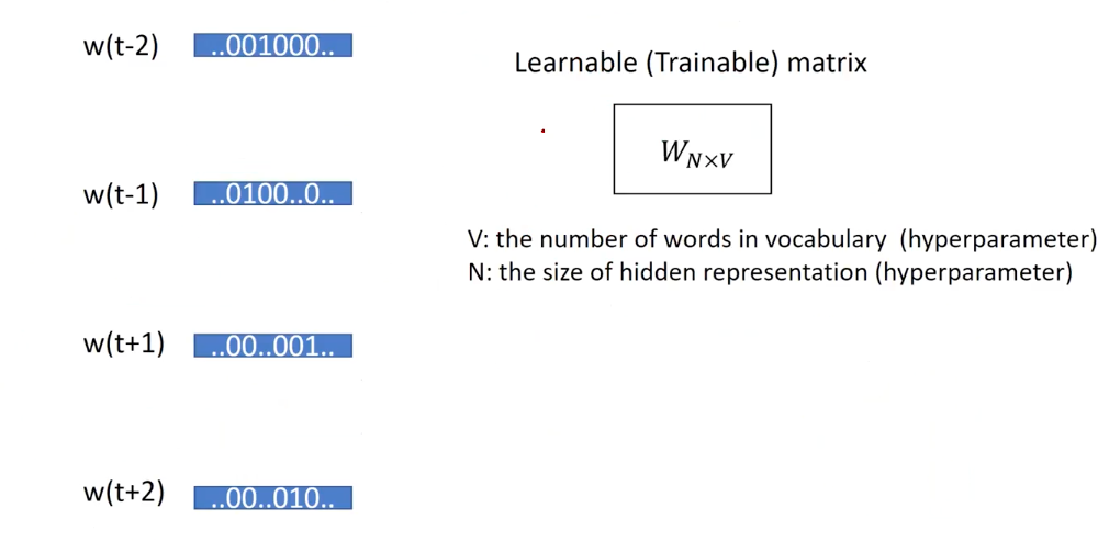
V is the vocabulary size (use e.g. 5000 words) and N is the window size (encode it e.g. 200 dimension!).

Let’s look at CBOW encoding process a little more formally.

1. Input: a set of one-hot vectors of given context words
2. Initialize a matrix for dimenstionality reduction.
3. Look up the hidden representations of context words.

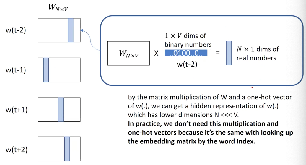
But on second thoughts, the W matrix is not one-hot, unless we set the dimension equal to the size of vocabulary. So, this CBOW is trying to overcome the (one-hot) sparse representation. It automatically finds dense representation in addition to contextual representation.

In practice, the (matrix)-(one-hot vector) multiplcation of ‘W’ times ‘a context word representation’ is always a vector in the vocabulary matrix, so they are basically same with the look up on cached matrix by their one-hot index. That is, what we’re doing in CBOW is to “look up the hidden representations of context words”

Why is it important? CBOW is faster than autoencoder, that’s why. They look-up layer is often called projection layer, requiring no activation function. Just doing look-up!

1. “Encode” into one hot represetnation and then “decode”
2. Then we get the vocabulary index for each target word

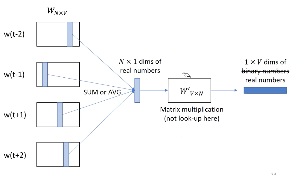
The big picture in CBOW is creating an aggregated vector that 1) represent the context of a word in a certain position via “look up” and 2) decode the hidden representation into the vocabulary dimension so that exact word can be obtained.

During the context word aggregation, we use mean operation conventionally.

What’s the difference against autoencoder?

Both are using encoder-decoder phases, but autoencoder is reconstructing the each word embedding in a reduced dimension, but CBOW is predicting a plausible target word in input context vectors, learning the encoder and decoder accordingly, benefitting from faster computation (lookup-in its encoder) and contextuality (“word semantic = cooccurence prob.” in its assumption).

How about CBOW training?

Compute a loss value and its gradients and backpropagate them for training. We use the softmax for activation and cross-entropy for loss function! Why? We are not reconstructing anything but predicting something, and softmax-entropy is a rule of thumb for that (if correct the entropy gets zero, which is ideal in information theory)

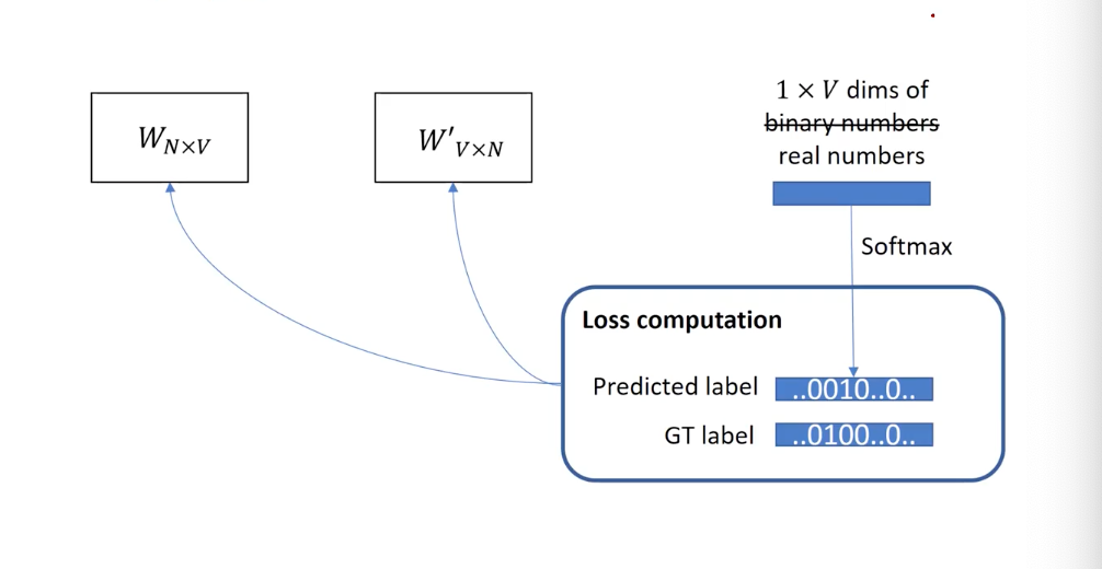
We train two matrix paramter, one is for look up (V->N) in the context encoding phase, and one is the opposite (N->V) in the decoding phase.

As the Word2Vec is trying to embed words just as autoencoder, we don’t really need the decoding matrix. We only need the encoder. Surprisingly, as we are modeling real-world word coocurrence to be encoded and decoded, the look up encoder in a well trained CBOW is usually quite similar to the transpose of the decoding matrix; converting vocabulary to hidden dimension <-> converting hidden dimension into vocabulary.

Word2Vec: Skip-gram

Skip-gram one of Word2Vec that is more popular than CBOW.

The difference between them is that the input is not context, but target word in skip-gram.

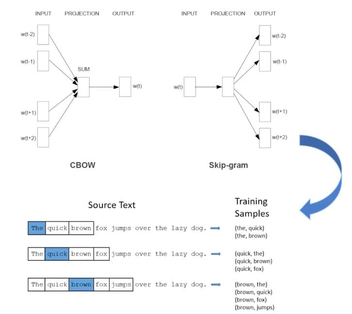
The sliding window for trainig sample colleciton is the same.

So given a sentence, the training samples can be the amount of possible target words in it. It’s kinda data augmentation. A better result from it, despite it’s more expensive in terms of computational costs.

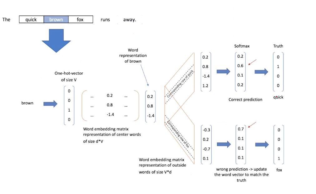
In its training, the two weight matrices are trained.

We basically get the hidden representation by target word embedding matrix (V->d). Then, given a window size, context word embedding matrix decode into higher dimension of vocaulary, as each of context words.

What’s the difference between CBOW and Skip-gram?

Predicting context words (CBOW) or target word (skip-gram) basically.

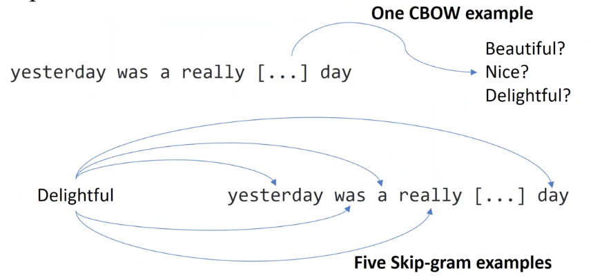
Skip-gram is more expensive, but higher in performance (accuracy) than CBOW.

CBOW: several times faster to train than the skip-gram, slighly better accuracy for the frequent words.

Skip-gram: works well with small amount of the training data, represents well even rare words or phrases. (More training samples in a corpus! More lines in the visual example.)

Word2Vec: other techniques

Computing the normalization factor is expensive: the softmax as activation function.

So they address this softmax cost issue by

1. Hierarchical Softmax
2. Negative Sampling

Look for the paper in Word2Vec paper for details.

Wrap up

1. Word embeddings: distributed representation of words.

2. Typically

   V

   > 10^6, 100 < d < 500!

3. One-hot vector -> feature vector
4. Fighting the curse of dimensionality with: compression (dimensionality reduction), smoothing (discrete to continuous), and densificaiton (sparse to dense)
5. Similar words end up close to each other in the feature space (contextual)

Word2Vec may be little hard, so as any other subject in deep learning. But note that AI studies pay off. Once you study something in AI and see the intuition behind it, you don’t easily forget them.

Teach yourself, ask a lot of questions to yourself/others. Clear understanding is the key, as they are accumulative.