Vanilla Feed-forward Neural Network

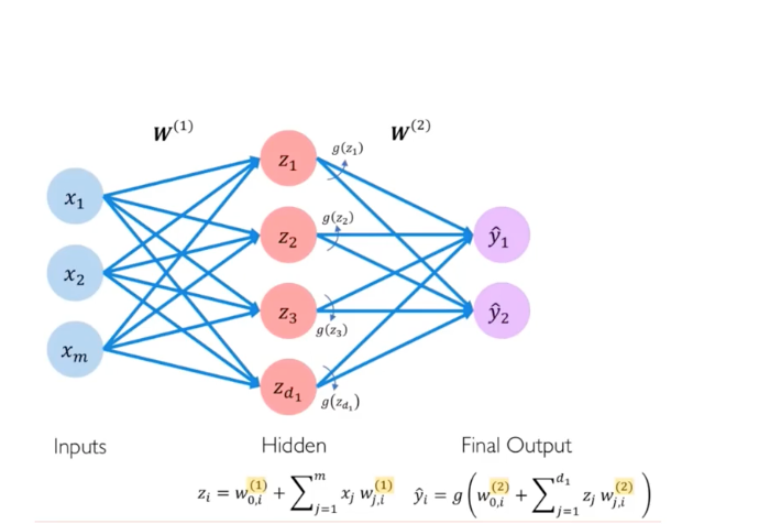
A vanilla feed forward network (FFN) recieves input with a fixed size (e.g. image), and the input is fed through hidden layers and produces outputs.

In a simplified way, FFNs are abtracted into layer levels: input layer, hidden layers, and output layer.

Vanilla FFNs are usually used to learn from sets of samples to induce labels.

How can we handle sequential data?

Sometimes mere sets of samples to train a model is my not be enough.

Samples are may not just indepednent and identically distributed (iid).

There are may be sequetial dependence among the samples.

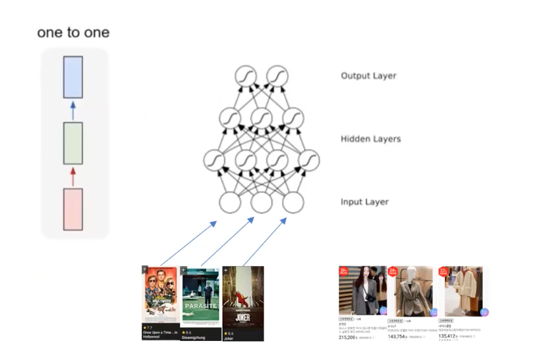
In movies, online shopping or speech recognition, the task goal is to predict what is the next given a historical information? e.g. Youtube recommendation based on your watch histories.

FFN for Sequential data

1. What if the length of sequential data is not fixed? Input, hidden, and output (red, green, blue recktangle) architecture cannot handle input of variable length.

2. Also, the order of such sequence may be very useful, but do FFNs can see the order?

A naive approach.

For issue #1, aggregation some groups of sequential data such as averaging the some partial sequence of data, converting variable-sized data into fixed-sized data in “Deep Neural Networks for YouTube Recommendations.”

However, some information in the data may be lost. That is, we may need to accumulate useful information that can be only seen through the ordering pattern of sequential samples.

Process Sequences

Features in many tasks have temporal/sequential dependencies.

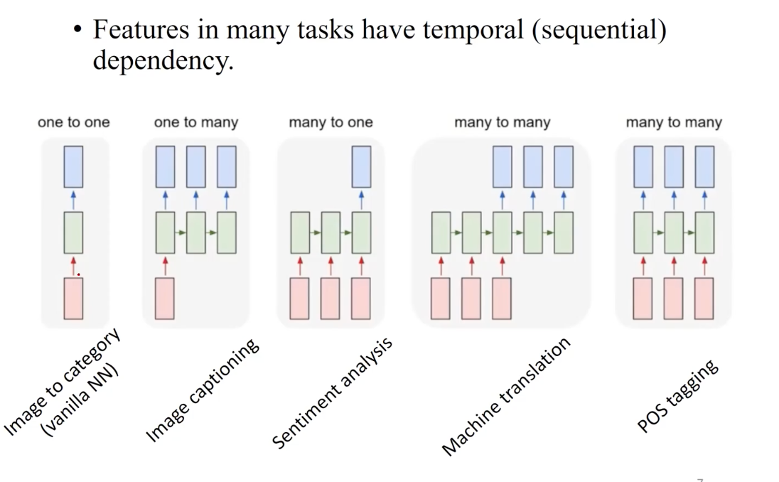
For the example tasks, from left to right,

1. one-to-one: FFN such as MNIST. Their input/output length has a fixed form. e.g. image size as input and class label as output.
2. one-to-many: here, the input length is fixed, but the output length is variable, e.g. image captioning, movie-to-genre.
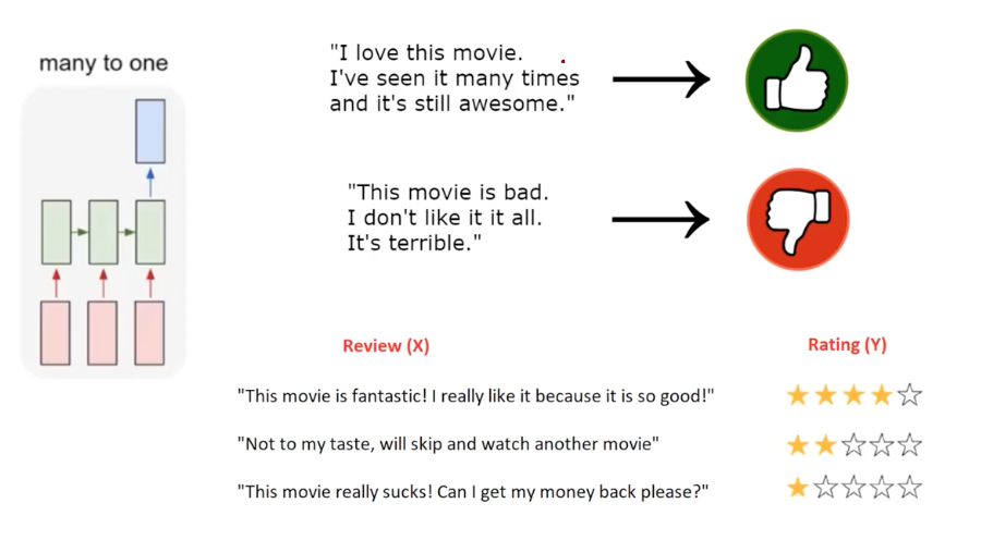
3. many-to-one: variable length input for one fixed-sized output. e.g. only the input for sentiment anlaysis is sequential text data (language input).
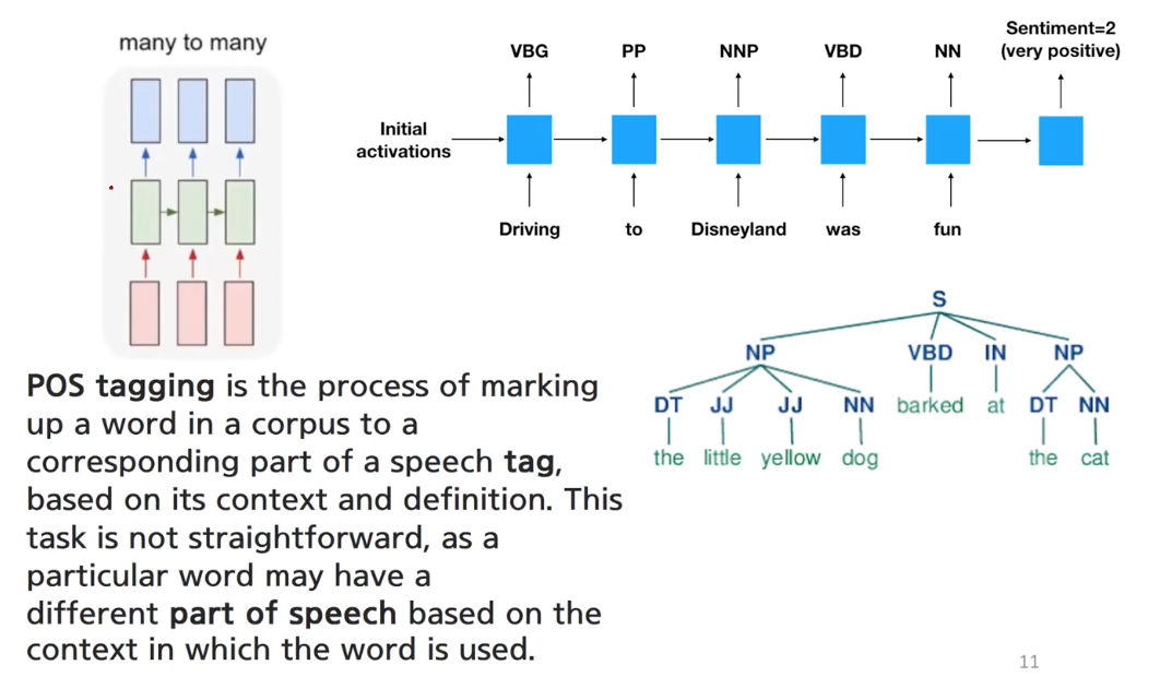
4. many-to-many: both input/output of variable length (they many not have the same length), e.g. machine translation, POS tagging.

Image Captioning

Image encoding (CNN) + language model (RNN)

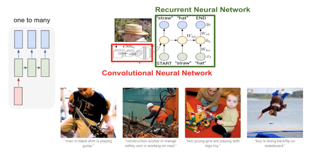
A famous dataset is MS COCO. This is not object detection! The caption is not one of class, but a variable-length sequence of texts. Very hard to solve this task.

Sentiment Analysis

A review text is given, classifcy into a finte set of class.

Machine Translation

Source language -> target language (e.g. Korean -> English)

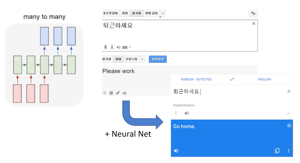
A huge leap in NNs: Google translate, Naver Papago.

Part-of-speech (POS) Tagging/Parsing

Marking a word in a sentence by its role (speech tag).

Improve model’s understanding on the language itself.

But recent language models are not that relying on such tagged information.

Recurrent Neural Networks

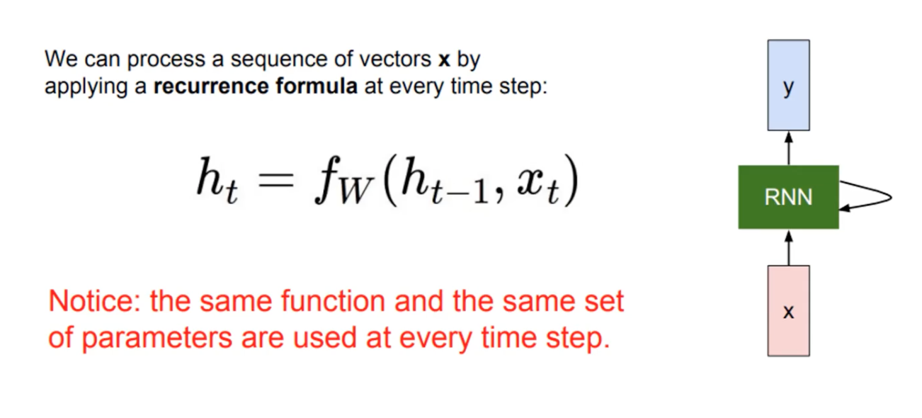
RNNs use one single module that encodes information given a time/position in temporal/sequential data.

So in each neuron of RNN, the output of the previous time step is fed as input of the next time step.

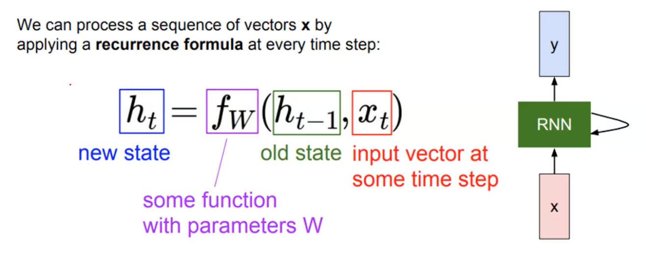
The abstract form of RNNs can be written as the above, where sequeces of input is process following the timestep t, and also preserving the old state to accumulate the inter-sample information.

The recurrence formulara shows processing the input and accumulated information to update newly aggregated information.

So it is aggregating the hidden state along every timestep following the flow of time (or sequence order).

Note that we are using the same function & parameters here.

Then, the question is what is the functional form and model architecture?

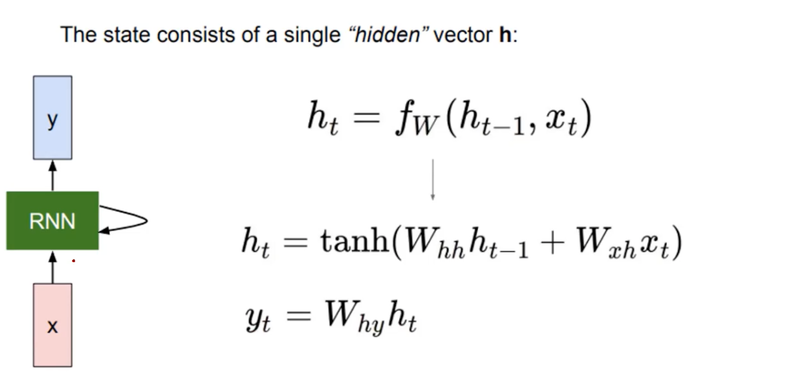
The W weight matrices and hidden representations are in the same variable that is used across the timesteps.

Here, W_hh encodes the hidden representation that is updated previously, and the W_xh the new input, sharing the model capacity to the past information and current input.

The reason to seperate two trainable wight matrices for hidden representation h_(t-1) and time-spceifc text x_(t) is 1) h and x are might not be of the same dimension 2) each weight matrix gets different roles of learning to map contextual content h and the textual content x. That is we give flexible learning room to the RNN models by giving explicitly seperating two heterogeneous inputs. We give the neural model an experince of individually embedding over more various type of input.

Also, tangent hyperbolic is used as non-linearity. They have output intervals from -1 to 1, which is more suitable in a hidden layer. However, we prefer sigmoid or softmax in the classification layer as they have the intervals from 0 to 1, which is good because it forms a probabilitic distribution like ground-truth labels, but not good for the hidden layers as they create vanishing gradient problems (the make hidden representation to be zeroed more and more). However, hyperbolic tangent or ReLU is relatively robust to vanishing gradient issue. In NLP, we see more of tanh than ReLU, whereas in Computer Vision, they prefer ReLU. The reason may be that the images in general requires partial information, which ReLU is known to be effective at.

The last linear layer W_ht are the final classification layer after the non-linearity.

Computational Graph for RNNs?

TO understand, just unroll the recursion in RNNs.

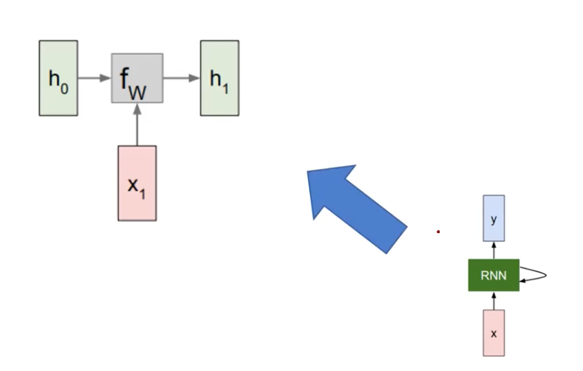
The current time is t=1. The current input is x_1, where the original input was h0 (initialized by some function). Update the h_0 to h_1, reflecting the new input in the sequence.

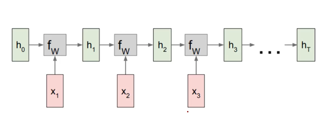
And repeat the process, until the sequence ends at t=T.

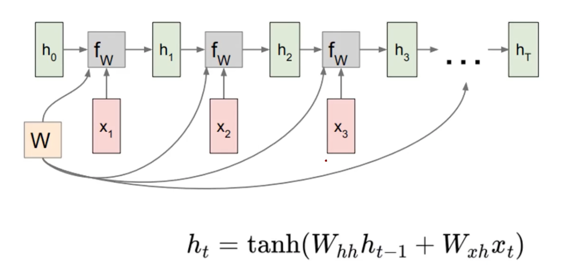
The most important thing is to keep the weight matrix W be a single variable that is responsible encoding and hence be the updated as the training target.

For example, a text sequence data “I am happy” and current time is 2 (embedding “happy”). Without considering the “I am” that came before encoding the “happy”, the target word would not be making a good sense. So we use the W weight matrix across time, they are learning the aggregation accross the time.

Mana to Many

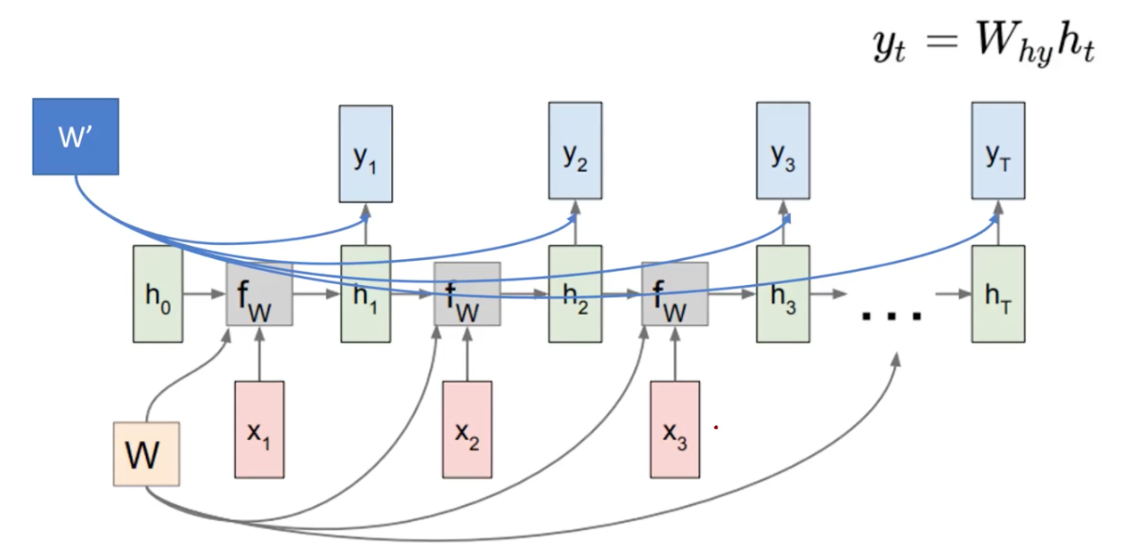
You can use encoder decoder architecture by employing another weight matrix W’. That is, we can use the h_t for the downstream task, that uses another set of parameters for the target task. (e.g.language model)

However, the computation is not cheap here. The more time passes, backpropagation would be increasing.

The Training

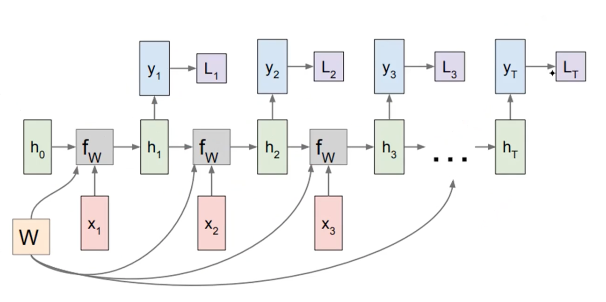
The label at each time step is given to supvervise the shared weight matrices. Then the entire loss would be the sum of individual losses, that is L1 ~ LT.

Many to One

This scenario assumes tasks like sentiment analysis. The target size is fixed, not of variable length.

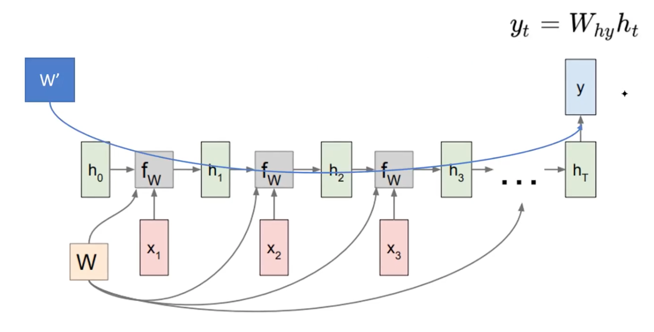
We read the sequence till the end, and the only hidden representation at the final time step is used. That is we assume the variable size information is all aggregated into the final representation.

Take a Closer Look

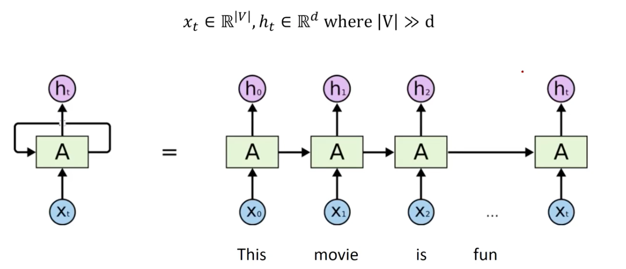
We can understand the mechanism of RNN as a dimensionality reduction.

In this figure the input at every timestep is a word in the vocabulary (actually its corresponding word embedding i.e. Word2Vec). At each timestep, the output is a hidden representation for the input word, reduced in the dimension size. That said, note that

V

is way bigger than d.

Then the projection into lower dimension is done by textual input embedding layer of W_{x, h}:

V

-> d and contextual input embedding layer of W_{h, h}: d -> d.

Studying backpropagation in RNNs is quite complex. Studying them would not worth the effort, as the first step would be to understand the general backpropagation in LMs or SOTA models.

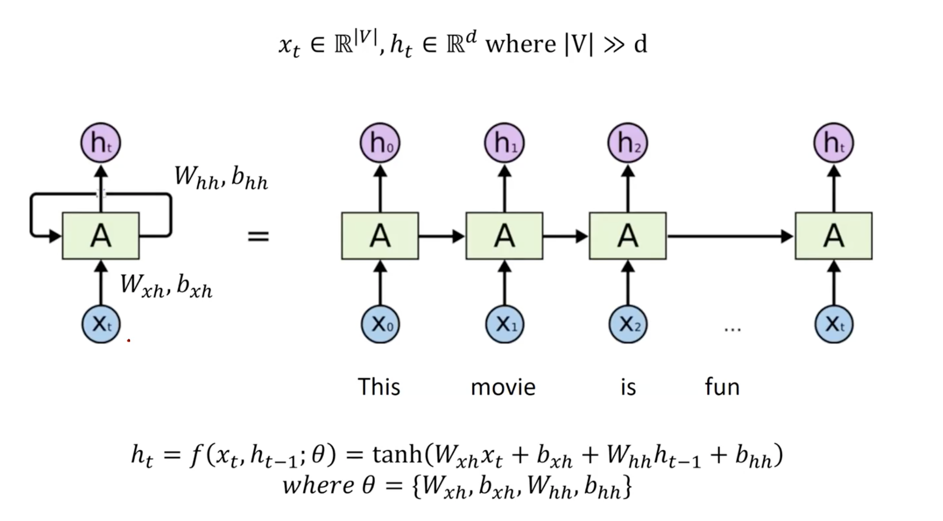
The text and context are processed via two independent linear layers for x and h, with non-linearity of hyperbolic tangent.

RNNs for NLPs

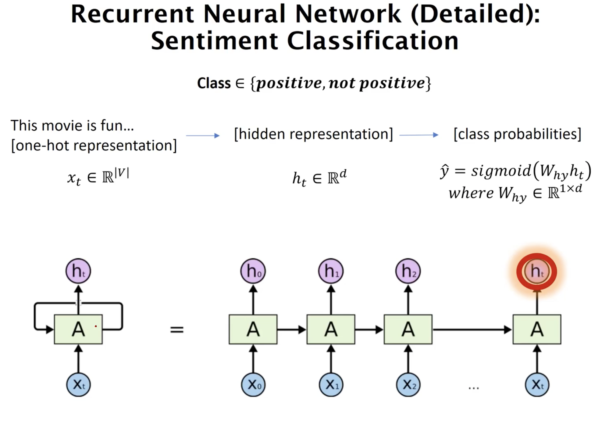
Following the represenation space projection from the input one-hot word indices, through hidden representation space, and ultimately into ther class propbability, one thing to note here is that, in the many-to-one scenario in sequential data such, a classification layer is attached only at the last timestep. In the sentiment classification, the output dimension is 2 (binary classification between positive and negative).

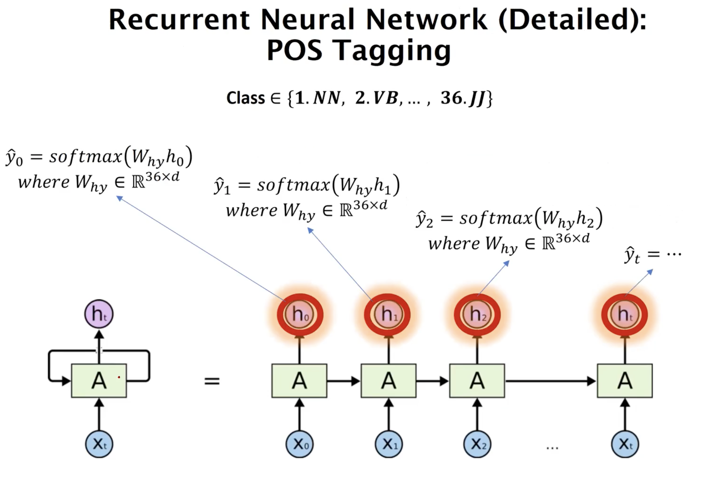
In one of many-to-many cases like POS tagging, the hidden state at every timestep is classified for downstream task. In this example, the number of class is 36.

Long Short Term Memory (LSTM)

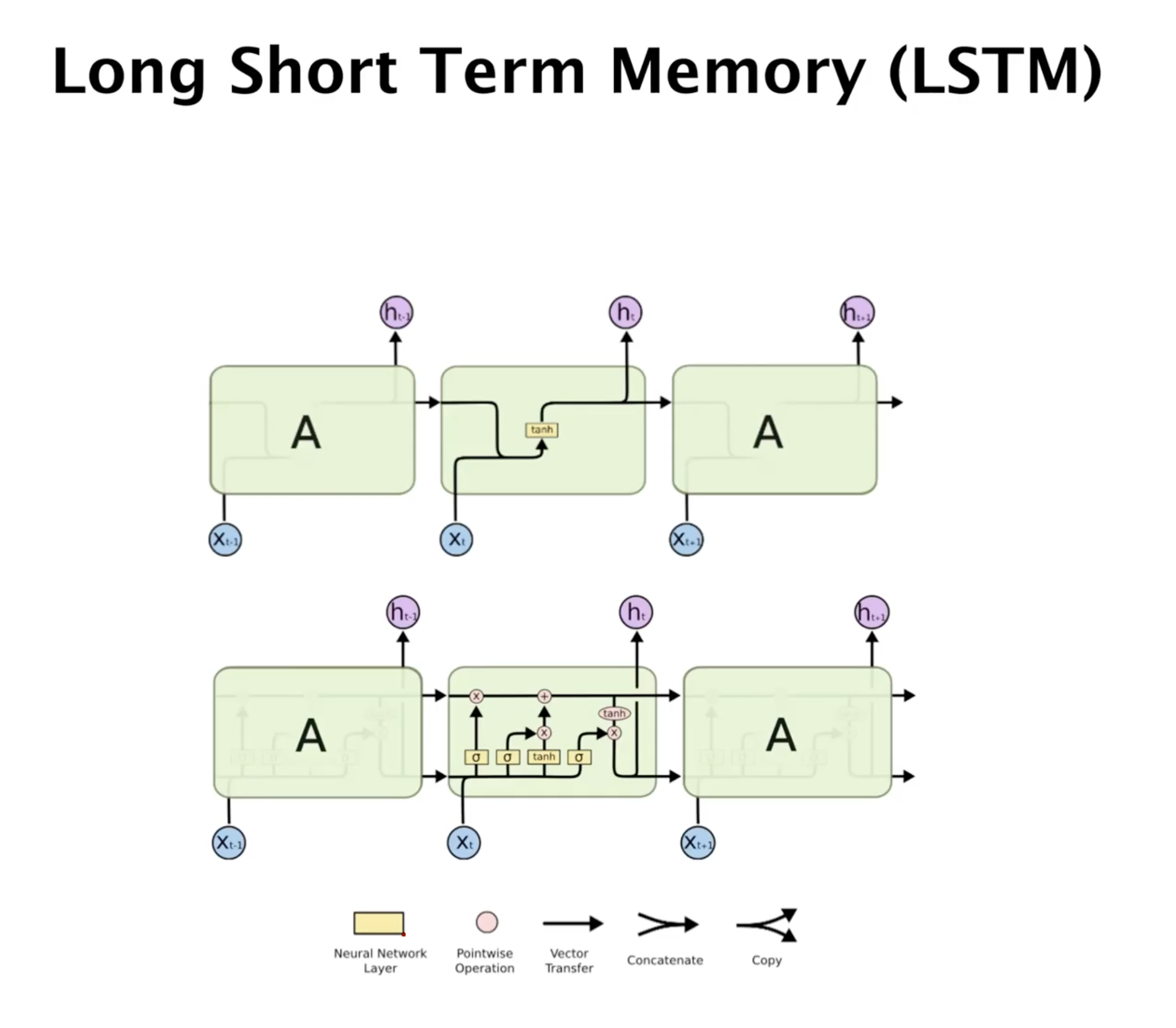
All recurrent models carry contextual information along the sequence of data, but in LSTM, instead of having a single unit in each cycle of recurrence, they use 4 different units, each interacting in an unique way. In the figure above, the upper recurrent units represent RNN, and the below shows LSTM. The skyblue circles are inputs at corresponding timestamp, and the pink dots are the hidden representations. Each yellow boxes are neural network layers, in which a set of trainable parameters are employed along with the denoted activation functions.

These gates allow LSTM to selectively add or remove information across the recurrent process. In RNNs, there is no such mechanism, as they can only pass the full information along the timestep. The 4 types of gates decide which per-time information is manipulated, where they add new information as a learning experience or remove some information to forget.

Why do we need to forget, and when do we use LSTMs? As an example, think of a person who speaks but murmurs. “I, I, I, .., I, I like movies”, an utterance may be given to RNNs. Then repeated, irrelavant parts of “I, I, I, .., I, I” should be automatically processed some how to reduce the importance of such parts, as the main semantics are about the speaker’s preference on the movie as a hobby. In long sequece of textual data, this ability to reduce the text span of irrevance gets more important.

In general, LSTMs are not that strong. They use relatively small amount parametes. The more lengthy the sequence of data gets, they show poor performance. However, they are very inspiring in how to use NNs to process the time dependent data flow.

Cell State

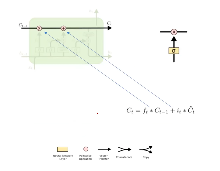
The key idea in LSTMs are to sense the data as a memory in computer science. The horizontal line in the diagram represents a memory “cell” that stores information. The stored information is called cell state. What is the difference between hidden representation and cell state? Unlike the hidden representation that is updated in a RNN way, where the whole information from the past is passed to the next block (the green box at each timestep), the cells are processed like a machine by the small neural network, called “gates”, that work as some sort of computer unit in the data processing circuit. The cell representation is carefully manipulated and updated to perserve only the relavant part of information, interpreted and interacted in the form of latent embedding (meaning they are just some sort of numerical vectors).

The pointwise operation (pink operation) and arrows show some kind of circuit board on a semi-conductive silicon that is hard-coded to efficient process temporal information, “cell state”. Units in LSTM architecture serves 4 functions: forgetting, learning, and updating cell state.

Specifically, the forgetting-and-learning relavant part of such circuits of the LSTMs are marked above, where a high-level explanation for the update process of cell states are drawn. To implement the forgetting, they use 0-to-1 weighting by multiplication over the past information C_{t-1} and use addition of new information embedding. As LSTMs weight the information in the previous memory cell storages, being not to forget, but to remember all when the weights are 1 (positive), the forgetting actually decides, not the degree of forgetting, but the degree of retaining the memory. But, we refer “forgetting” regarding its purpose of selectively removing some temporal information.

Forget and Input Gates

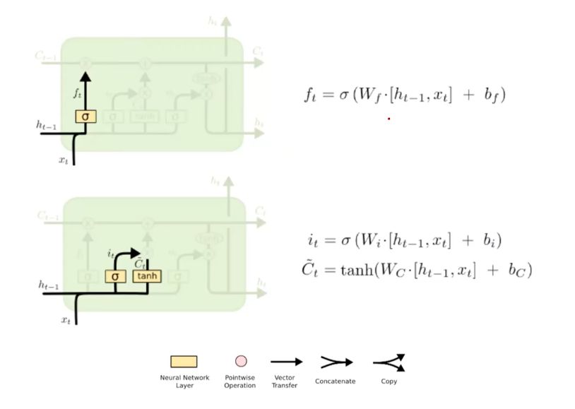
The forget function is implemented by the neural parameters W_f, b_f in the first block. The learning function is done by the W_i, b_i, where they use the input at newly learned data at the time t. That is, the information in the memory cells are process in a hardcoded firmware that these two forget/input gates are supposed to learn to efficiently update them.

Specifically, beside the work of the input gates, where it decides the importance of current input data, LSTMs employed another layer W_c, b_c that prepares a informational increment (denoted as C_tilda) that serves as update patch content based on the current input. This gate only considers the hidden representation and current input, and not the previous cell states, to prepare an update patch of new inforamtion for the previous cell state. They use tanh as a activation function so that the the update patch forms the range between -1 and 1, representing both additive and reductive properties of new experience. Being negative in the new cell state increment doesn’t mean they forget. Tanh allows rather more manipulative updates, being not only positive but also negative values.

However, these are just architectural choices, where no standard answer is set. What’s important in LSTMs is that data in cells can be, and should be, processed to be seletively preserved.

Updating Cell State

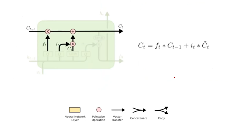
The way to update the previous cell state is very simple. Given the selectively forgotten (retained) cell state based on the weighting (multiplcation) over the previous cell state, and the selectively forgatten cell state based on the weighting over the current cell state (C_tilda), we only need to add them. We already prepared the positive-negative forms of state update patch in prior (W_c, b_c).

Output Gates

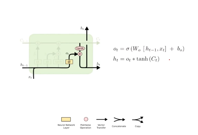
Finally, we decide what to output as the t-time result of recurrent update on the sequential data. This result will be based on the updated cell state. Given a cell state, the output-related meachinsm in LSTM decide between the updated cell state and the input of current timestep t. This also is done through the multiplication-based weighting over the cell state, where the weights are learned end-to-end (hence output gate) based on the current input. Note that the cell state is activated by tanh function (-1 ~ 1) so that its expressivity increases.

What we’re doning in this stage is the reason why we keep both cell state and hidden representation. The goal of LSTM is not only solving the task, but also deciding what to remember and what to forget. To address this information selection, LSTM address this by decoupling 1) hidden representation as the reference variable and 2) cell state as the resultant variable, where the resultant variables are iteratively updated based on the input reference variables. That is, hidden representations are defining the cell states at each time.

How do we initialize all the units in RNNs or LSTMs? Random initialization of very small weights.