In this post, we discuss the sequence-to-sequence (seq2seq) model, and attention mechanism. Actually, attention mechanism was proposed based on the seq2seq models.

Applications of RNNs

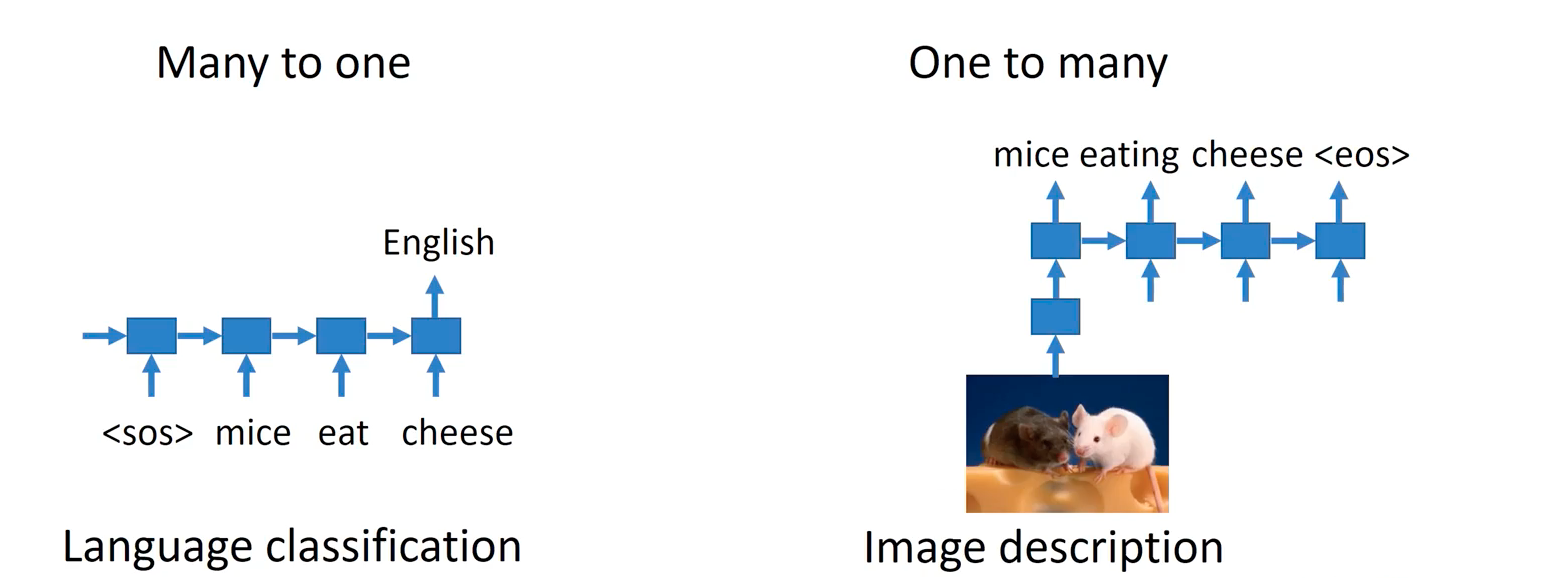
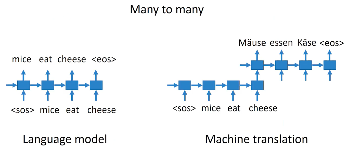
We discussed NLP tasks that require processing the sequential data in the previous posts. Recently, we handle sequential data of longer length that requires complex reasoning and natural language understanding. Especially in many-to-many sequential data, things are a lot tougher.

RNN Language Model

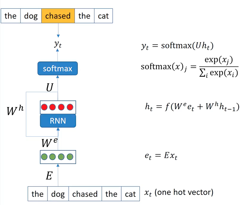
We’re showing the RNN used as the language model. What’s a language model (LM)? But for now, think of it as a model that predicts the most probable word, next to an arbitrary sentence. That is, LM tasks aim to train a model that learns a language pattern. Given a sequence of words as input (e.g. “The dog chased the cat”), at each position, we need to predict the word in the next poisition following it. Previously, we regarded a word input as a one-hot embedding or an index in a vocabulary. However, in here, a Word2Vec embedding is used as the basic format of input for the RNNs, where it outputs a prediction of most probable word out of whole vocabulary. Note that we employ a word embedding layer multiplied to the one-hot input embedding of certain word (e_t = E * x_t). Furthermore, depending on the application, we could let the word embedding layer (E) to be trainable or frozen, choosing to use the naive pretrained embedding or more tuned embedding to the target corpus. The recurrence allows RNNs to update the self-contextual hidden representation over each word. Usually, the final output should be in the probability space, so they takes the softmax function as the last activation function. We minimize the distance between prediction distribution size and one-hot representation, both of which have the dimension size of the vocabulary size. One may use a cross-entropy.

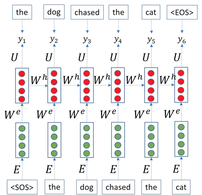
Here, the recurrent process of RNNs is horizontally unrolled along the time dimension. Starting with a sepcial token <\SOS> (abbr. for the start of sentence), The process repeat until the model output <\EOS> token (the end of sentence).

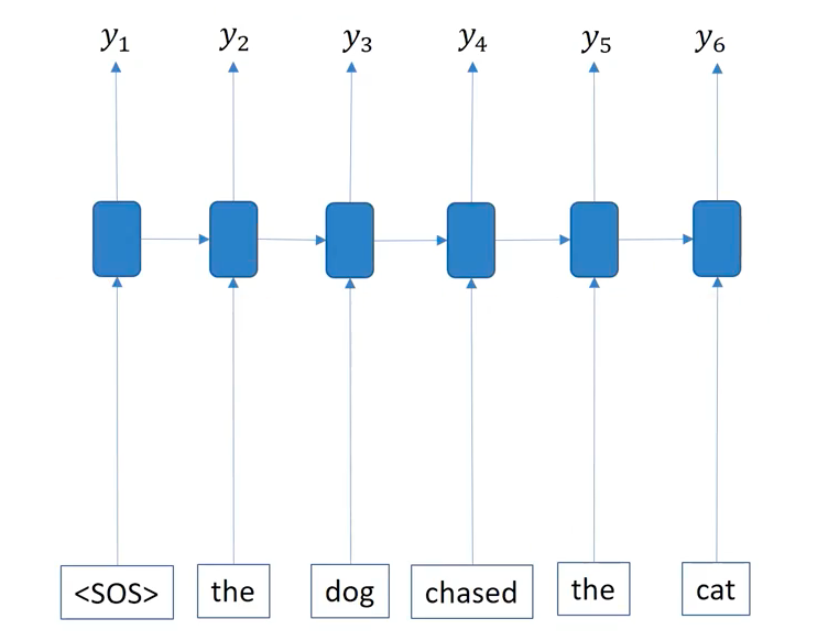
Inducing a more simplified diagram of the recurrent process in RNNs, we need to be able to think of the inner RNNs module in the blue box, that is ommitted in practical descriptions.

Multi-layer RNN LM

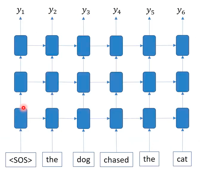
What if we attach a new RNN module that takes the output of another RNN module? By stacking RNNs, we could use a multi-layer RNN LMs that have a deeper model architecture than normal RNNs. Don’t forget that the horizontal block is a RNN module at different timestep.

Why would we need a multi-layer RNNs for LM task? For sure, we want to improve the LMs. One may argue that the size of increasing the training data may be better than increasing the depth of the network. It’s reasonable doubts that employing a deeper network often result in the overfitting. But, what’s the key difference between language model task and text classification task? The main difference is that text classification is supervised learning but langauge model is a unsupervised learning. For LMs, there are nearly unlimited amount of data available. With such sufficient amount of data (of course not labeled, but ok becasue we’re just predicting the next word in a sentence), we are relatively safe to build a model with more parameters without worrying the overfting issue.

RNNs for Translation

The translation above turns a sentence of 5 English words in to 7 French words. As the sentence length differs between in the source language and in the target language, machine translation needs to handle mappings between sequences of different length. We use sequence-to-sequence model for that. Its a many-to-many type of sequntial data processing, where it has a variable length for two sequences.

Encoder-decoder Model

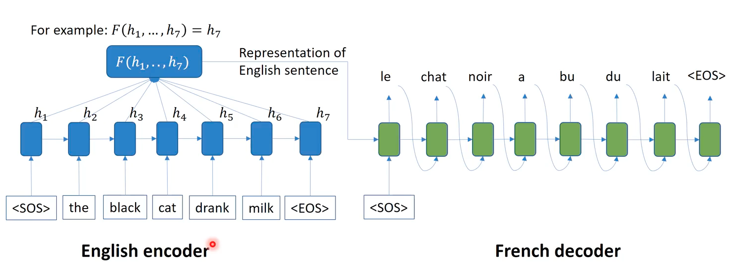
The encoder-decoder model is a hypernym of seq2seq model. In this picture, we have two RNNs unrolled as each of color blue and greed, where the former first encode an English sentence into a hidden representation and the latter decode it into a French sentence. Specifically, we get the hidden representation of fixed length, by aggregating all hidden representation at each time. Simply we could just use the last hidden representation (h_7) as the aggregated representation, called “context” vector. The decoder takes this context and <\SOS> as input, and repeats taking its output as input, producing a probable word as output in sequence, until the <\EOS>. Note that encoder-decoder arhchitecture is quite fleixbile; for example in image captioning task, people usually use CNNs as the encoder and use the texutal RNNs as the decoder. Using RNNs that can process a sequence of arbitrary length, encoder-decoder models were successful in many tasks.

During training a encoder-decoder model, the decoder produces the output at each timestep. These outputs are the words having the maximum probability at each timestep. We’re taking the best guess of the model, and supervise the model to learn to predict the groud-truth sequence in the training dataset. Here, we use what’s called a teacher forcing technique, which corrects an error in a sequence to prevent the error propagation along the sequence. When a decoder fails to predict the correct word, teacher forcing provides the ground-truth word as input to the next RNN module, instead of incorrectly predicted word, so that the model gets chances to continue learning based on a sensible information. Optimizing based on the sum of each word’s errors, the back-propagation is applied from the last time in the decoder to the first word in the encoder.

Greedy Inference

During inference time, we cannot apply the teacher forcing, as the ground truth words are not known. The input at each decoding time is the one-hot vector for word with the max softmax probability from the previous step. At least, we’re converting a probabilitic distribution of prediction into one-hot representation here.

Beam Search

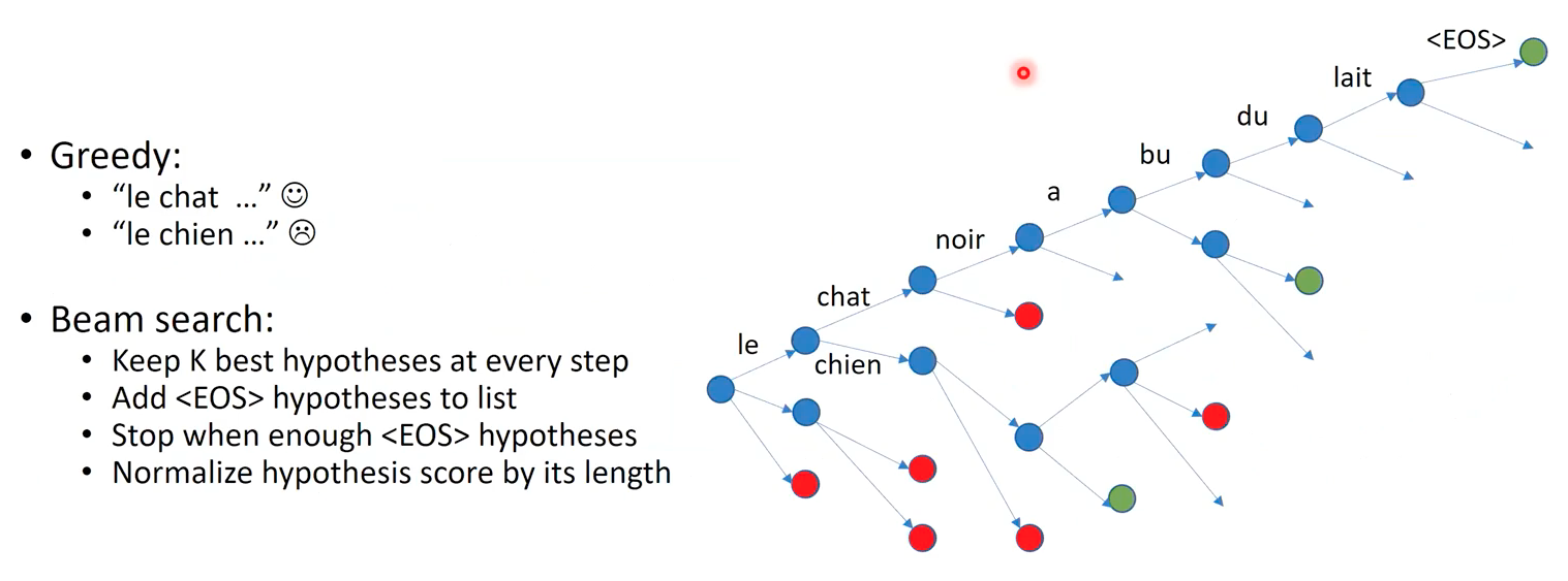
Let’s assume a situation where at a specific time of decoding stage, the model needs to decide between two words that are very similar (i.e. chat vs chien at time t=2). Their embedding representation is also very similar. If the decoder choose a incorrect word (chien in the example), then the prediction is errorneous already (at time 2). To prevent this from the beginning, the beam search aims to create and keep multiple probable sentences as alternative candidate for the final answer.

Specifically, in this decoding strategy, they keep K best hypotheses at every step. Imagine a bunch of metal beams lying on the floor. The pile of beams have a fixed width and are stacked vertically in the shape of parallel lines. Here in beam search, we maintain top-K possible answer sentences just like those beams. Referring a predicted word as a hypotheis at each timestep, the hypotheses forms paths of blue nodes in the tree on the right side of the image, where each node indicates a word that take a part in a candidate sentence. That is, starting with the first word “le” as the root node in the tree, beam search at each depth prepends several child nodes to a existing (previously predicted) node, where each new word makes up a root-to-leaf sentence. Along the timesteps, only K paths that has the highest probability can extends their childs. That is, we always keep several amount of candidate sentences. Regarding all such active sentence paths, if a <\EOS> is attached as the most probable hypothesis, we regard that path is finished, considered as a finished answer candidates.

Greedy search vs beam search? Emprically compare them out.

Limitation of Encoder-Decoder Model

Each decoder time step depends on the same encoder embedding (context vector). Encoder embedding is assumed to hold the information for every encoder time step, and has the responsibility to summrize into the fixed sized dimension. The problem is that unlike the fixed size of the context vector, the encoder may have variable length, may have enormously long sequence to encode. It would sometimes be impossible to encode all the information in a long sentence into relatively tiny vectors, even though we employ LSTMs to select the most important parts. The descrepancy between the sentence length and the context length may create a bottleneck to recurrent models. No matter how long the text we train the model in training time, there can be longer text in test time, casuing drop in model performance.

Attention Mechanism

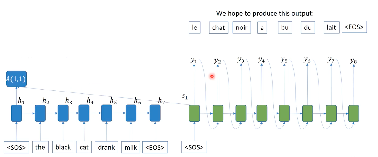
Forget about the final aggregation of hidden representations in the previous encoder-decoer model. We are not aggregating the temporal information into a context vector. Instead, we replace it by attention mechanisme, that considers which words to focus to at each time based on the relavance, as subset of words will substitue to serve as useful contextual information. This mechanism calculates importance weights of each word embedding in the prepared by the encoder in parallel, given a hidden representation at each timestep during the decoding stage. This calculation is done by neural networks, called attention layers, that identifies which words are important depending on the input vector being decoded.

In other words, think of a search engine. When we search about something via Google, the web browser send the query about the thing you ask (i.e. the winner of Oscar), the server returns relavant documents that may be useful to you. By the relavance in attention mechanism, usually this means similarity between the queried embedding and the returned embedding.

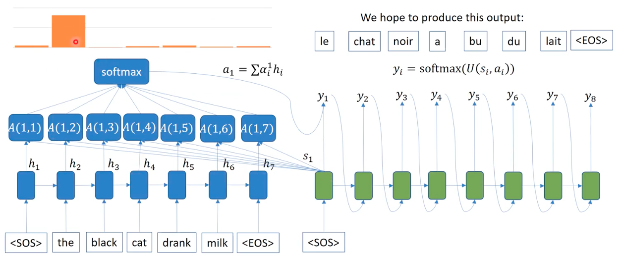
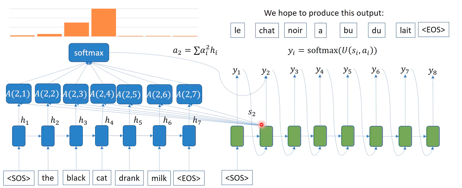
Specifically, depending on the queried word embedding at time t in decoding phase, attention mechanism caculates each embedded words in the source sentence, convert them into probabilitic weights via softmax function, and rewieght the each word embeddings according to the weights. Summing up all the attention-importance weighted embeddings, at time s_1, we could see that the word “the” is the most important word for “<\SOS>”, where decoder takes such aggregated embedding (a_1 = sum of alpha_i x h_i) as input (a_i) in addition to the hidden representation of the previous output (s_i). Unlike a single context vector in RNNs, the attention makes context vectors (a_i) at each decoding time. Note that the input of attention is not the word at the decoding timestep, it is the context vector that include the target word at time t, which is based on the output of the previous step.

Types of Attention

There are diverse types of attention methods, regarding how to compute the similarity between two words. However, note that this similarity may not corresponds to the human sense of similarity, as it is learned by a machine which has no human biases but is optimized in its own manner.

The first attention uses dot product to compute the similarity. So in this approach, two hidden representations in the encoding and decoding phases must have the same dimensionality.

The second attention uses a multiplcation of weight matrix to project the decoding embedding into the same space of the encoding embedding. Unlike the dot product based attention, this attention mechanism may be consisdered as a small sized neural network as it possess trainable parameters on its own.

The third attention is called additive attention, where both embeddings are projected into a space of the same dimesion, and then be added. In this setting, tanh is usually used as the activation fucntion.

There are many other approaches. Generally attention mechanism aligns the input and output sequences, and compute the similarity scores for the pair.